2 Theory

2.1 Exact kernel density estimation

Given a set of $n$ sample points $x_k$ ($k = 1,\cdots,n$), an exact kernel density estimation $\widehat{f}_h(x)$ can be calculated as

\[\begin{equation} \widehat{f}_h(x) = \frac{1}{nh} \sum_{k=1}^n K\Big(\frac{x-x_k}{h}\Big) \tag{2.1} \end{equation}\]

where $K(x)$ is called the kernel function, $h$ is the bandwidth of the kernel and $x$ is the value for which the estimate is calculated. The kernel function defines the shape and size of influence of a single data point over the estimation, whereas the bandwidth defines the range of influence. Most typically a simple Gaussian distribution ($K(x) :=\frac{1}{\sqrt{2\pi}}e^{-\frac{1}{2}x^2}$) is used as kernel function. The larger the bandwidth parameter $h$ the larger is the range of influence of a single data point on the estimated distribution.

The computational complexity of the exact KDE above is given by $\mathcal{O}(nm)$ where $n$ is the number of sample points to estimate from and $m$ is the number of evaluation points (the points where you want to calculate the estimate). There exist several approximative methods to decrease this complexity and therefore decrease the runtime as well.

2.2 Binning

The most straightforward way to decrease the computational complexity is by limiting the number of sample points. This can be done by a binning routine, where the values at a smaller number of regular grid points are estimated from the original larger number of sample points. Given a set of sample points $X = \{x_0, x_1, ..., x_k, ..., x_{n-1}, x_n\}$ with weights $w_k$ and a set of equally spaced grid points $G = \{g_0, g_1, ..., g_l, ..., g_{n-1}, g_N\}$ where $N < n$ we can assign an estimate (or a count) $c_l$ to each grid point $g_l$ and use the newly found $g_l$ to calculate the kernel density estimation instead.

\[\begin{equation} \widehat{f}_h(x) = \frac{1}{nh} \sum_{l=1}^N c_l \cdot K\Big(\frac{x-g_l}{h}\Big) \tag{2.2} \end{equation}\]

This lowers the computational complexity down to $\mathcal{O}(N \cdot m)$. Depending on the number of grid points $N$ there is tradeoff between accuracy and speed. However as we will see in the comparison chapter later as well, even for ten million sample points, a grid of size $1024$ is enough to capture the true density with high accuracy¹⁰. As described in the extensive overview by Artur Gramacki¹¹ simple binning or linear binning can be used, although the last is often preferred since it is more accurate and the difference in computational complexity is negligible.

2.2.1 Simple binning

Simple binning is just the standard process of taking a weighted histogram and then normalizing it by dividing each bin by the sum of the sample points weights. In one dimension simple binning is binary in that it assigns a sample point’s weight ($w_k = 1$ for an unweighted histogram) either to the grid point (bin) left or right of itself.

\[\begin{equation} c_l = c(g_l) = \sum_{\substack{x_k \in X\\\frac{g_l + g_{l-1}}{2} < x_k < \frac{g_{l+1} + g_l}{2}}} w_k \tag{2.3} \end{equation}\]

where $c_l$ is the value for grid point $g_l$ depending on sample points $x_k$ and their associated weights $w_k$.

2.2.2 Linear binning

Linear binning on the other hand assigns a fraction of the whole weight to both grid points (bins) on either side, proportional to the closeness of grid point and data point in relation to the distance between grid points (bin width).

\[\begin{equation} c_l = c(g_l) = \sum_{\substack{x_k \in X\\g_l < x_k < g_{l+1}}} \frac{g_{k+1}-x_k}{g_{l+1} - g_l} \cdot w_k + \sum_{\substack{x_k \in X\\g_{l-1} < x_k < g_l}} \frac{x_k - g_{l-1}}{g_{l+1} - g_l} \cdot w_k \tag{2.4} \end{equation}\]

where $c_l$ is the value for grid point $g_l$ depending on sample points $x_k$ and their associated weights $w_k$.

2.3 Using convolution and the Fast Fourier Transform

Another technique to speed up the computation is rewriting the kernel density estimation as convolution operation between the kernel function and the grid counts (bin counts) calculated by the binning routine given above.

By using the fact that a convolution is just a multiplication in Fourier space and only evaluating the KDE at grid points one can reduce the computational complexity down to $\mathcal{O}(\log{N} \cdot N)$.¹¹

Using the equation (2.2) from above only evaluated at grid points gives us

\[\begin{equation} \widehat{f}_h(g_j) = \frac{1}{nh} \sum_{l=1}^N c_l \cdot K\Big(\frac{g_j-g_l}{h}\Big) = \frac{1}{nh} \sum_{l=1}^N k_{j-l} \cdot c_l \tag{2.5} \end{equation}\]

where $k_{j-l} = K(\frac{g_j-g_l}{h})$.

If we set $c_l = 0$ for all $l$ not in the set $\{1, ..., N\}$ and notice that $K(-x) = K(x)$ we can extend equation (2.5) to a discrete convolution as follows

\[\begin{equation} \widehat{f}_h(g_j) = \frac{1}{nh} \sum_{l=-N}^N k_{j-l} \cdot c_l = \vec{c} \ast \vec{k} \tag{2.6} \end{equation}\]

where the two vectors look like this

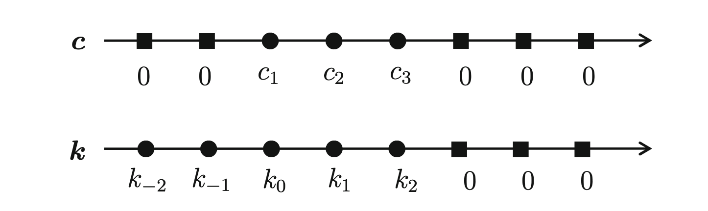
$Vectors $\vec{c}$ and $\vec{k}$ used for the convolution$

Figure 2.1: Vectors $\vec{c}$ and $\vec{k}$ used for the convolution

By using the well known convolution theorem we can fourier transform $\vec{c}$ and $\vec{k}$, multiply them and inverse fourier transform them again to get the result of the discrete convolution.

However, due to the limitation of evaluating only at the grid points themselves, one needs to interpolate to get values for the estimated distribution at points in between.

2.4 Improved Sheather-Jones Algorithm

A different take on KDEs is described in the paper ‘Kernel density estimation by diffusion’ by Botev et al.¹² The authors present a new adaptive kernel density estimator based on linear diffusion processes which also includes an estimation for the optimal bandwidth. A more detailed and extensive explanation of the algorithm as well as an implementation in Matlab is given in the ‘Handbook of Monte Carlo Methods’¹³ by the original paper authors. However the general idea is briefly sketched below.

The optimal bandwidth is often defined as the one that minimizes the mean integrated squared error ($MISE$) between the kernel density estimation $\widehat{f}_{h,norm}(x)$ and the true probability density function $f(x)$, where $\mathbb{E}_f$ denotes the expected value with respect to the sample which was used to calculate the KDE.

\[\begin{equation} MISE(h) = \mathbb{E}_f\int [\widehat{f}_{h,norm}(x) - f(x)]^2 dx \tag{2.7} \end{equation}\]

To find the optimal bandwidth it is useful to look at the second order derivative $f^{(2)}$ of the unknown distribution as it indicates how many peaks the distribution has and how steep they are. For a distribution with many narrow peaks close together a smaller bandwidth leads to better result since the peaks do not get smeared together to a single peak for instance.

As derived by Wand and Jones an asymptotically optimal bandwidth $h_{AMISE}$ which minimizes a first-order asymptotic approximation of the $MISE$ is then given by¹⁴

\[\begin{equation} h_{AMISE}(x) = \Big( \frac{1}{2N\sqrt{\pi} \| f^{(2)}(x)\|^2}\Big)^{\frac{1}{5}} \tag{2.8} \end{equation}\]

where $N$ is the number of sample points (or grid points if binning is used).

As Sheather and Jones showed, this second order derivative can be estimated, starting from an even higher order derivative $\|f^{(l+2)}\|^2$ by using the fact that $\|f^{(j)}\|^2 = (-1)^j \mathbb{E}_f[f^{(2j)}(X)], \text{ } j\geq 1$

\[\begin{equation} h_j=\left(\frac{1+1 / 2^{j+1 / 2}}{3} \frac{1 \times 3 \times 5 \times \cdots \times(2 j-1)}{N \sqrt{\pi / 2}\left\|f^{(j+1)}\right\|^{2}}\right)^{1 /(3+2 j)} = \gamma_j(h_{j+1}) \tag{2.9} \end{equation}\]

where $h_j$ is the optimal bandwidth for the $j$-th derivative of $f$ and the function $\gamma_j$ defines the dependency of $h_j$ on $h_{j+1}$

Their proposed plug-in method works as follows:

Compute $\|\widehat{f}^{(l+2)}\|^2$ by assuming that $f$ is the normal pdf with mean and variance estimated from the sample data
Using $\|\widehat{f}^{(l+2)}\|^2$ compute $h_{l+1}$
Using $h_{l+1}$ compute $\|\widehat{f}^{(l+1)}\|^2$
Repeat steps 2 and 3 to compute $h^{l}$, $\|\widehat{f}^{(l)}\|^2$, $h^{l-1}$, $\cdots$ and so on until $\|\widehat{f}^{(2)}\|^2$ is calculated
Use $\|\widehat{f}^{(2)}\|^2$ to compute $h_{AMISE}$

The weakest point of this procedure is the assumption that the true distribution is a Gaussian density function in order to compute $\|\widehat{f}^{(l+2)}\|^2$. This can lead to arbitrarily bad estimates of $h_{AMISE}$, when the true distribution is far from being normal.

Therefore Botev et al. took this idea further¹². Given the function $\gamma^{[k]}$ such that

\[\begin{equation} \gamma^{[k]}(h)=\underbrace{\gamma_{1}\left(\cdots \gamma_{k-1}\left(\gamma_{k}\right.\right.}_{k \text { times }}(h)) \cdots) \tag{2.10} \end{equation}\]

$h_{AMISE}$ can be calculated as

\[\begin{equation} h_{AMISE} = h_{1}=\gamma^{[1]}(h_{2})= \gamma^{[2]}(h_{3})=\cdots=\gamma^{[l]}(h_{l+1}) \tag{2.11} \end{equation}\]

By setting $h_{AMISE}=h_{l+1}$ and using fixed point iteration to solve the equation

\[\begin{equation} h_{AMISE} = \gamma^{[l]}(h_{AMISE}) \tag{2.12} \end{equation}\]

the optimal bandwidth $h_{AMISE}$ can be found directly.

This eliminates the need to assume normally distributed data for the initial estimate and leads to improved performance, especially for density distributions that are far from normal as seen in the next chapter. According to their paper increasing $l$ beyond $l=5$ does not increase the accuracy in any practically meaningful way. The computation is especially efficient if $\gamma^{[5]}$ is computed using the Discrete Cosine Transform - an FFT related transformation.

The optimal bandwidth $h_{AMISE}$ can then either be used for other kernel density estimation methods (like the FFT-approach discussed above) or also to compute the kernel density estimation directly using another Discrete Cosine Transform.

2.5 Using specialized kernel functions and their series expansion

Lastly there is an interesting approach described by Hofmeyr¹⁵ that uses special kernel functions of the form $K(x) := poly(|x|) \cdot exp(−|x|)$ where $poly(|x|)$ denotes a polynomial of finite degree.

Given the kernel with a polynom of order $\alpha$

\[\begin{equation} K_{\alpha}(x) := \sum_{j=0}^{\alpha} |x|^j \cdot e^{−|x|} \tag{2.13} \end{equation}\]

the kernel density estimation is given by (equation (2.1))

\[\begin{equation} \widehat{f}_h(x) = \frac{1}{nh} \sum_{k=1}^{n}\sum_{j=0}^{\alpha} (\frac{|x-x_k|}{h})^{j} \cdot e^{(-\frac{|x-x_k|}{h})} \tag{2.14} \end{equation}\]

where as usual $n$ is the number of samples and $h$ is the bandwidth parameter.

Hofmeyr showed that the above kernel density estimator can be rewritten as \[\begin{equation} \widehat{f}_h(x) = \sum_{j=0}^{\alpha}\sum_{i=0}^{j} {j \choose i}(\exp (\frac{x_{(\tilde{n}(x))}-x}{h}) x^{j-i} \ell (i, \tilde{n}(x))+\exp (\frac{x-x_{(n(x))}}{h})(-x)^{j-i} r(i, \tilde{n}(x))) \tag{2.15} \end{equation}\]

where $\tilde{n}(x)$ is defined to be the number of sample points less than or equal to $x$ ($\tilde{n}(x) = \sum_{k=1}^{n} \delta_{x_{k}}((-\infty, x])$, where $\delta_{x_{k}}(\cdot)$ is the Dirac measure of $x_k$) and $\ell(i, \tilde{n})$ and $r(i, \tilde{n})$ are given by

\[\begin{equation} \ell(i, \tilde{n})=\sum_{k=1}^{\tilde{n}}(-x_{k})^{i} \exp (\frac{x_{k}-x_{\tilde{n}}}{h}) \tag{2.16} \end{equation}\]

\[\begin{equation} r(i, \tilde{n})=\sum_{k=\tilde{n}+1}^{\tilde{n}}(x_{k})^{i} \exp (\frac{x_{\tilde{n}} - x_{k}}{h}) \tag{2.17} \end{equation}\]

Or put differently, all values of $\widehat{f}_h(x)$ can be specified as linear combinations of terms in $\bigcup_{i, \tilde{n}}\{\ell(i, \tilde{n}), r(i, \tilde{n})\}$. Finally, the critical insight lies in the fact that $\ell(i, \tilde{n})$ and $r(i, \tilde{n})\}$ can be computed recursively as follows

\[\begin{equation} \ell(i, \tilde{n}+1)=\exp(\frac{x_{\tilde{n}}-x_{\tilde{n}+1}}{h}) \ell(i, \tilde{n})+(-x_{\tilde{n}+1})^{i} \tag{2.18} \end{equation}\]

\[\begin{equation} r(i, \tilde{n}-1)=\exp(\frac{x_{\tilde{n}-1}-x_{\tilde{n}}}{h})(r(i, \tilde{n})+(x_{\tilde{n}})^{i}) \tag{2.19} \end{equation}\]

Using this recursion one can then calculate the kernel density estimation with a single forward and a single backward pass over the ordered set of all $x_{\tilde{n}}$ leading to a computational complexity of $\mathcal{O}((\alpha+1)(n+m))$ where $\alpha$ is the order of the polynom, $n$ is the number of sample points and $m$ is the number of evaluation points. What is important to note here is that this is the only method that defines a computational gain for an exact kernel density estimation. Although we can also use binning to approximate it and reduce the computational complexity even further, it is already a significant runtime reduction for the exact estimate.