5 Comparison

To compare the efficiency and performance of the different kernel density estimation methods implemented with TensorFlow a benchmarking suite was developed. It consists of three parts: a collection of distributions to use, a collection of methods to compare and a runner module that implements helper methods to execute the methods to test against the different distributions and plot the generated datasets nicely.

The goal is to access whether the newly proposed methods (ZfitBinned, ZfitFFT, ZfitISJ and ZfitHofmeyr) are able to compete with current KDE implementations in Python in terms of runtime for a given accuracy. Furthermore the benchmarking between the four new implementations should yield insights to choose the right method for the right use case.

5.1 Benchmark setup

To compare the different implementations multiple popular test distributions mentioned in Wand et al.¹⁴ were used (see figure 5.1). A simple normal distribution, a simple uniform distribution, a bimodal distribution comprised of two normals, a skewed bimodal distribution, a claw distribution that has spikes, and one called asymmetric double claw that has different sized spikes left and right. This test distributions are implemented using TensorFlow Probability and data is sampled from each test distribution at random. The different KDE methods are then used to approximate this test distributions from the sampled data.

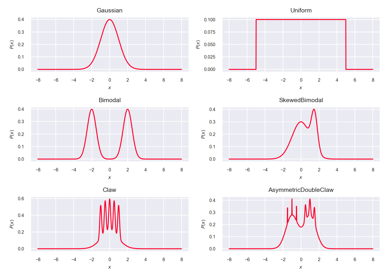
Figure 5.1: Test distributions used to sample data from

All comparisons were made using a standard Gaussian kernel function. Although all location-scale family distributions of TensorFlow Probability may be used for the new implementation proposed in this paper, the Gaussian kernel function is the most used one and provides best reference to compare different implementations against each other. An exception is ZfitHofmeyr (see 4.6), which uses a specialized kernel function of the form $poly(x)\cdot\exp(x)$, namely the $K_1$ kernel function with a polynom of order $\alpha = 1$ as given by equation (2.13). The $K_1$ kernel function is used, since it was shown to be the most performant in nearly all cases in Hofmeyr’s own benchmarking²². Indicating this and the fact that the underlying algorithm was implemented in C++ as a custom TensorFlow operation, the Hofmeyr method used in the comparisons is therefore appropriately called ZfitHofmeyrK1withCpp.

For all approximative implementations linear binning with a fixed bin count of $N = 2^{10} = 1024$ was used. This is the default in KDEpy, a power of $2$ (which is favorable for FFT based algorithms), results in an exact kernel density calculation for the lowest sample size used ($10^3$) but also yields results with high accuracy for the highest sample size used ($10^8$). Decreasing the bin count would decrease the runtime while providing lesser accuracy whereas increasing the bin count would yield higher accuracy while increasing the runtime (see 2.2). However, as all methods compared use the same linear binning routine, changing the bin count does not change how they compare. Therefore the bin size is kept fixed.

For nearly all implementations the bandwidth was calculated using the popular rule of thumb introduced by Silverman²³, because it is simple to compute and sufficient to capture the differences between implementations. The only exception is the ISJ based method, since it is based on calculating the approximately optimal bandwidth directly (as shown in section 2.4).

5.2 Differences of Exact, Binned, FFT, ISJ and Hofmeyr implementations

First, the exact kernel density estimation implementation is compared against the linearly binned, FFT and ISJ and Hofmeyr implementations run on a Macbook Pro 2013 Retina using the CPU.

The sample sizes lie in the range of $10^3$ to $10^4$. The number of samples is restricted because calculating the exact kernel density estimation for more than $10^4$ kernels is computationally unfeasible (larger datasets would lead to an exponentially larger runtime).

5.2.1 Accuracy

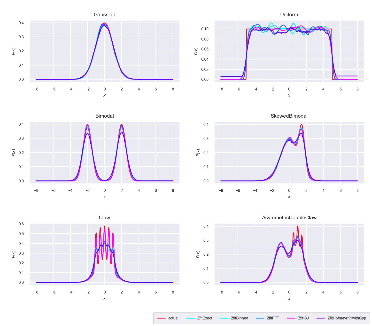
Figure 5.2: Comparison between the five algorithms ‘Exact,’ ‘Binned,’ ‘FFT,’ ‘ISJ’ and ‘Hofmeyr’ with $n=10^4$ sample points

As seen in figure 5.2, all implementations are capturing the underlying distributions rather well, except for the complicated spiky distributions at the bottom. Here the ISJ approach is especially favorable, since it does not rely on Silverman’s rule of thumb to calculate the bandwidth. This can be seen in figure 5.3 in more detail.

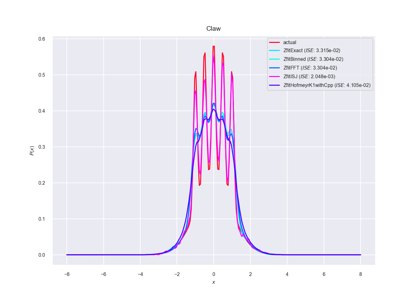
Figure 5.3: Comparison between the five algorithms ‘Exact,’ ‘Binned,’ ‘FFT,’ ‘ISJ’ and ‘Hofmeyr’ with $n=10^4$ sample points on distribution ‘Claw’

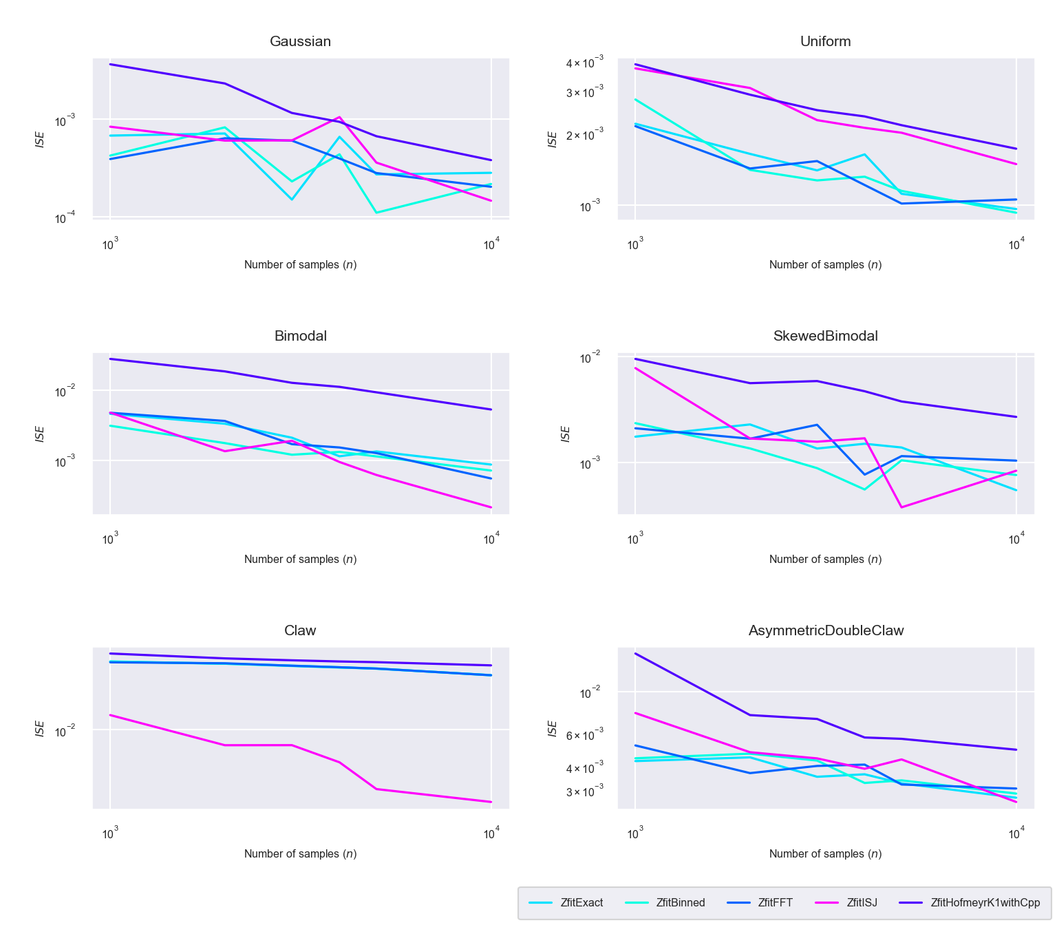
Figure 5.4: Integrated square errors ($ISE$) for the five algorithms ‘Exact,’ ‘Binned,’ ‘FFT,’ ‘ISJ’ and ‘Hofmeyr’

The calculated integrated square errors ($ISE$) per sample size can be seen in figure 5.4. As expected the $ISE$ decreases with increased sample size. The specialized kernel method (implemented as TensorFlow operation in C++: ZfitHofmeyrK1withCpp) has a higher $ISE$ than the other methods for all distributions. Although the ISJ based method’s (ZfitISJ) accuracy is equally as poor for the uniform distribution, it has the lowest $ISE$ for the spiky ‘Claw’ distribution, which confirms the superiority of the ISJ based bandwidth estimation for highly non-normal, spiky distributions. For other type of distributions the exact, linearly binned and FFT based method have comparable integrated square errors, which suggest that the the accuracy loss of linear binning is negligible compared to the exact kernel density estimate.

5.2.2 Runtime

The runtime comparisons are split in an instantiation and an evaluation phase. In the instantiation phase everything is prepared for evaluation at different values of $x$, depending on the method used more or less calculation happens during this phase. In the evaluation phase the kernel density estimate is calculated and returned for the evaluation points.

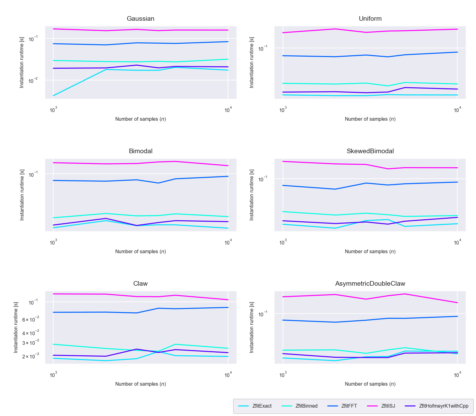
Figure 5.5: Runtime difference of the instantiaton phase between the five algorithms ‘Exact,’ ‘Binned,’ ‘FFT,’ ‘ISJ’ and ‘Hofmeyr’

As seen in figure 5.5, the FFT and ISJ method use more time during the instantiation phase than the other methods. This is expected, since for these methods the kernel density estimate is calculated for every grid point during the instantiation phase, whereas for the other methods, the calculation is only prepared and actually executed during the evaluation phase itself. In addition, we can see that the FFT method is faster than the ISJ method in calculating the kernel density estimate for the grid points. The linear binning method is slower than the exact method because the bin counts are calculated during the instantiation phase.

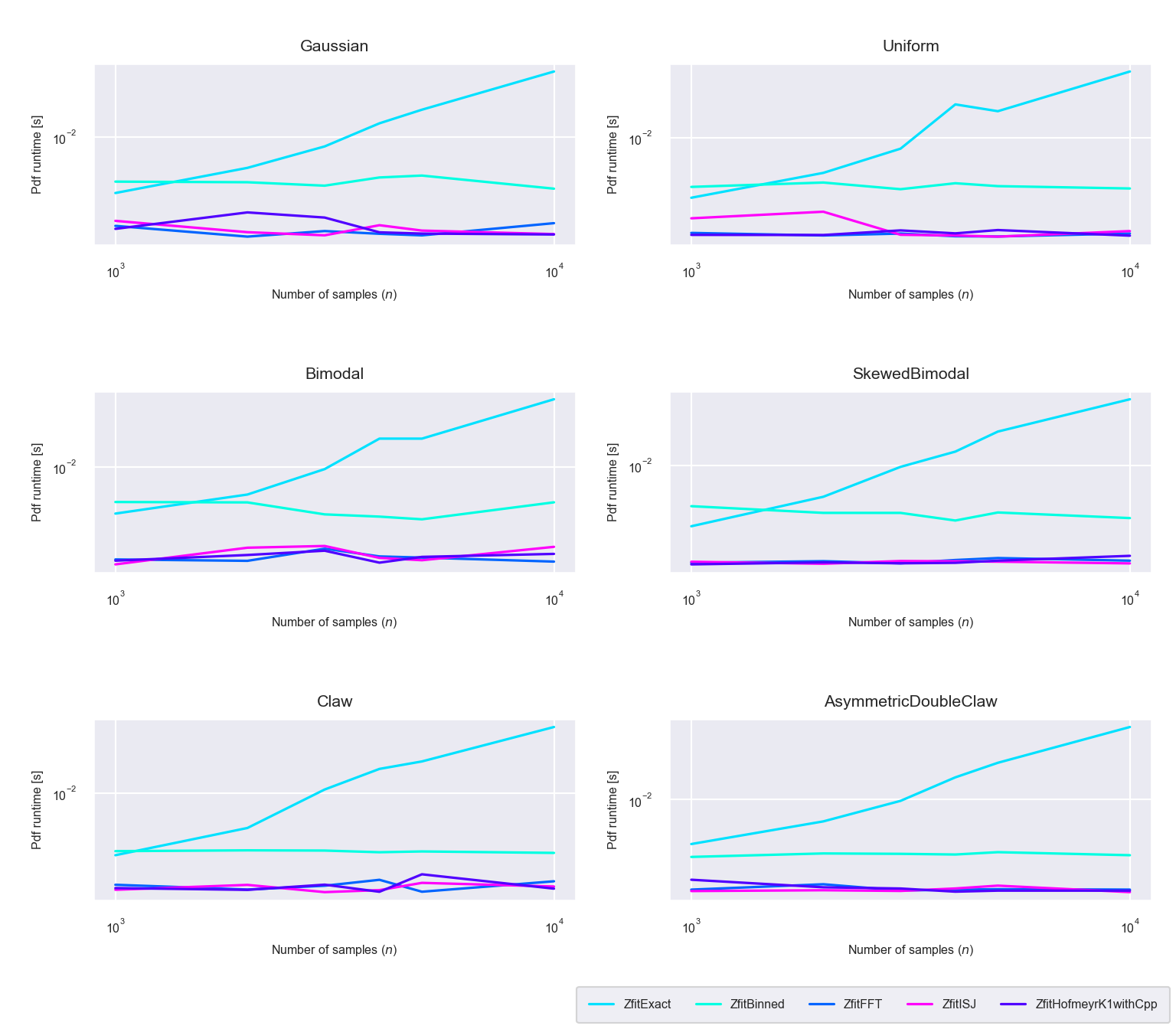
Figure 5.6: Runtime difference of the evaluation phase between the five algorithms ‘Exact,’ ‘Binned,’ ‘FFT,’ ‘ISJ’ and ‘Hofmeyr’

In figure 5.6 we can see that evaluation runtime of the exact KDE method increases with increased bin size, whereas for the other methods it stays nearly constant. The binned method benefits from the fact that, no matter how big the sample size is, it has to compute the kernel density estimate only for the fixed bin count of $N=1024$. The other methods are faster during the evaluation phase, because they have already calculated estimate in the instantiation phase and only need to interpolate for the values in between.

5.3 Comparison to KDEpy

Now the newly proposed methods (Binned, FFT, ISJ, Hofmeyr) are compared against the state of the art implementation in Python KDEpy, also run on a Macbook Pro 2013 Retina using the CPU. The number of samples per test distribution is in the range of $10^3$ - $10^8$. By excluding the exact kernel density estimation, larger sample data sizes can be used for comparison.

5.3.1 Accuracy

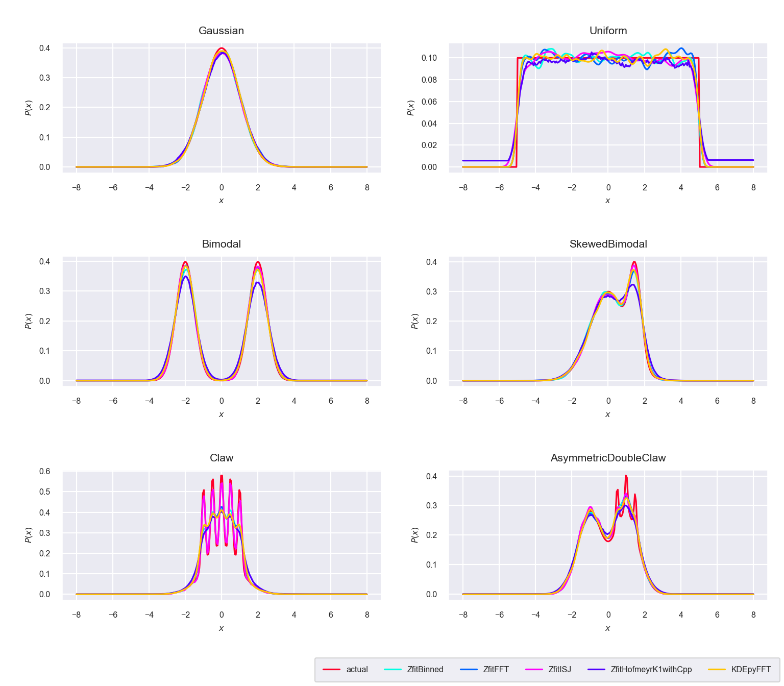
Comparison between the newly proposed algorithms 'Binned', 'FFT', 'ISJ', 'Hofmeyr' and the FFT based implementation in KDEpy with $n=10^4$ sample points

Figure 5.7: Comparison between the newly proposed algorithms ‘Binned,’ ‘FFT,’ ‘ISJ,’ ‘Hofmeyr’ and the FFT based implementation in KDEpy with $n=10^4$ sample points

The different methods show the same behavior as the reference implementation in KDEpy, again with the exception of the ISJ algorithm, which works better for spiky distributions (figure 5.7).

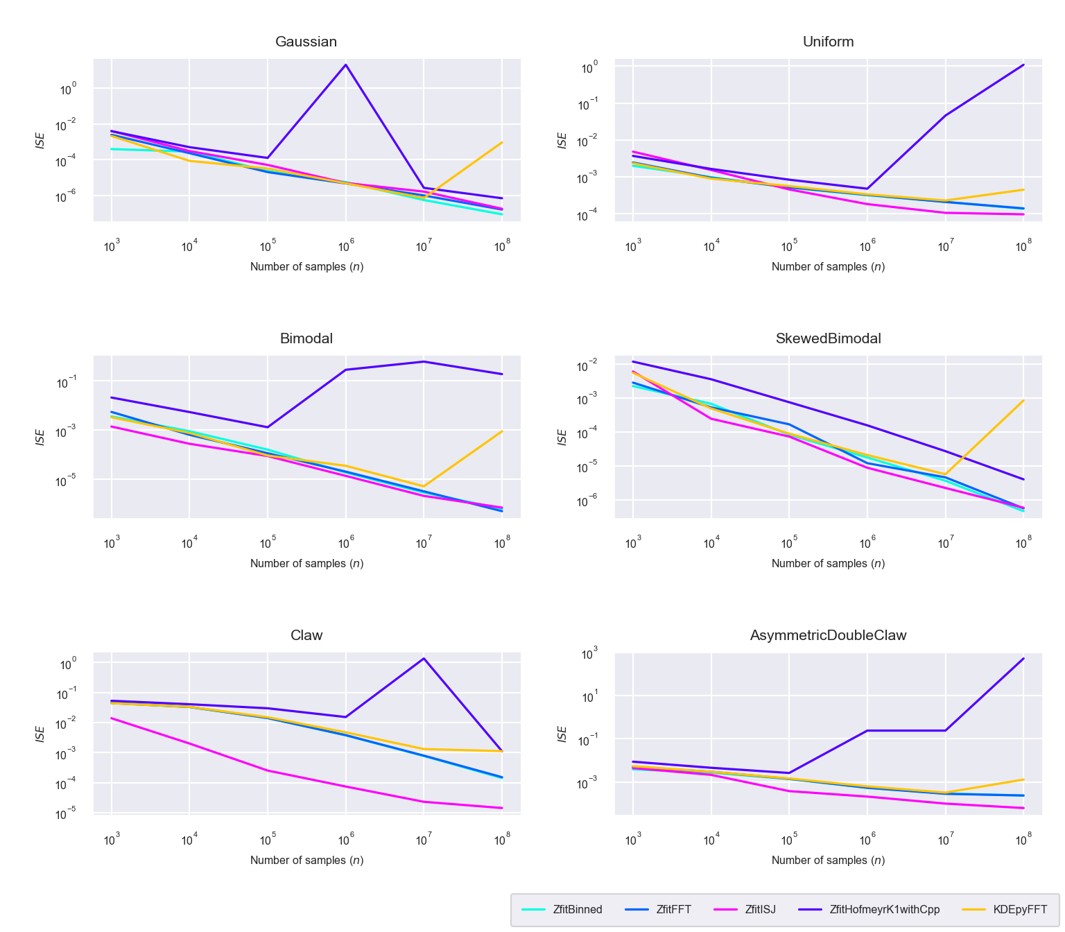
Figure 5.8: Integrated square errors ($ISE$) for the newly proposed algorithms ‘Binned,’ ‘FFT,’ ‘ISJ,’ ‘Hofmeyr’ and the FFT based implementation in KDEpy

The integrated square errors plotted in figure 5.8, are in general in the same order of magnitude for all implementations, except for the Hofmeyr method, which shows unrealistically high errors for higher sample sizes. This might relate to an uncaught overflow error in the custom TensorFlow operation implemented in C++ and should be investigated further. Additionally we see again that the ISJ method’s $ISE$ is an order of magnitude lower for the spiky ‘Claw’ distribution, because it calculates a bandwidth closer to the optimum and does not rely on assuming a normal distribution in doing so. It can be shown also that the binned, FFT and ISJ methods capture the nature of the underlying distributions with high accuracy using only $N = 2^{10}$ bins even for a sample size of $n = 10^8$. KDEpy’s FFT based implementation loses accuracy for higher sample sizes ($n \geq 10^8$), whereas the new binned, FFT and ISJ methods increase their accuracy even further, which suggests that using TensorFlow increases numerical stability for extensive calculations like kernel density estimations.

5.3.2 Runtime

Again the runtime comparisons are split in an instantiation and an evaluation phase.

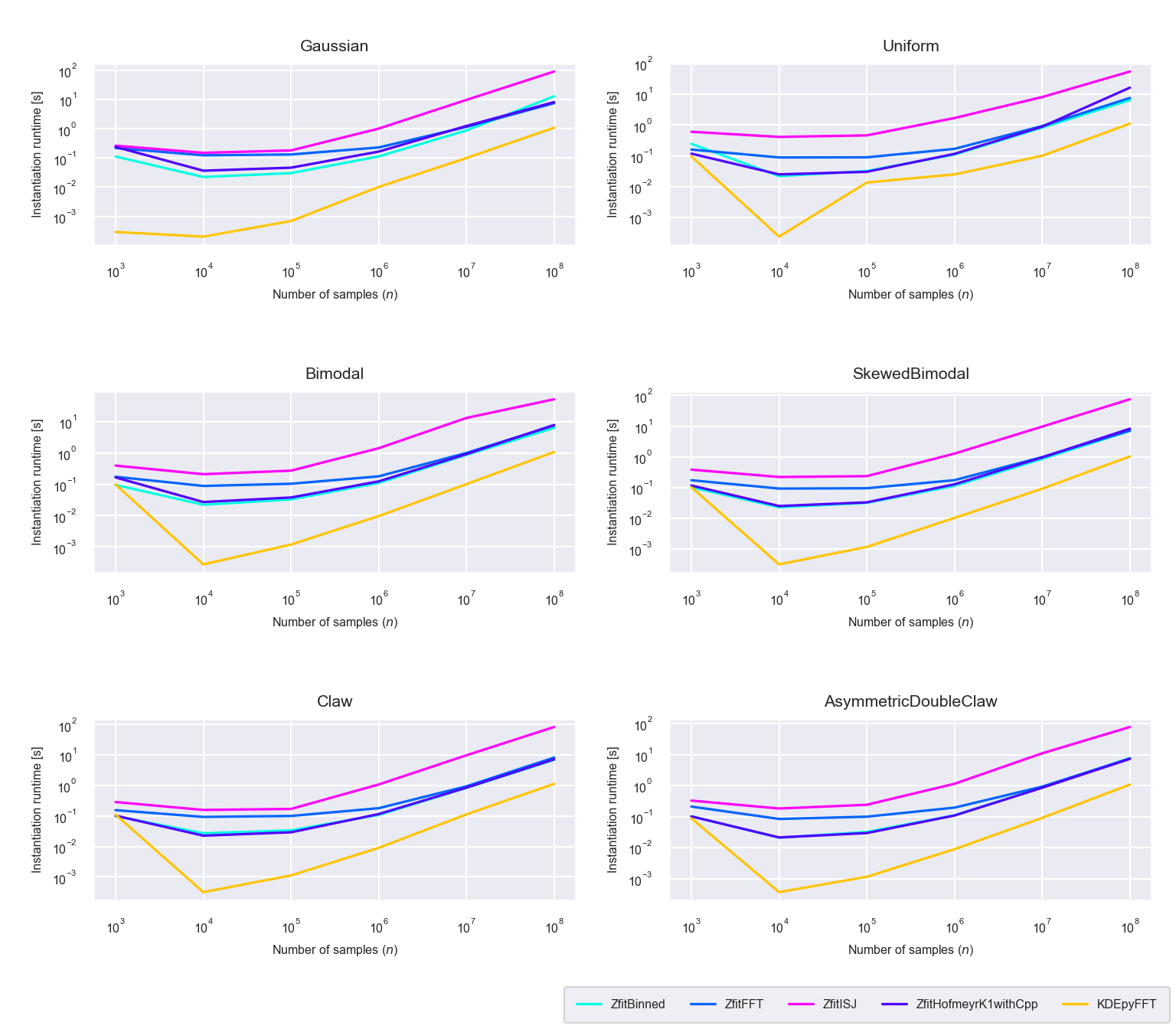
Runtime difference of the instantiaton phase between the newly proposed algorithms 'Binned', 'FFT', 'ISJ', 'Hofmeyr' and the FFT based implementation in KDEpy

Figure 5.9: Runtime difference of the instantiaton phase between the newly proposed algorithms ‘Binned,’ ‘FFT,’ ‘ISJ,’ ‘Hofmeyr’ and the FFT based implementation in KDEpy

During the instantiation phase the newly proposed binned, FFT, ISJ and Hofmeyr methods are slower than KDEpy’s FFT method by one or two orders of magnitude (figure 5.9). This is predictable, since generating the TensorFlow graph generates some runtime overhead.

In many practical situtations in high energy physics however, generating the TensorFlow graph and the PDF has to be done only once and the PDF is evaluated repeatedly. This is for instance important if using the distribution estimate for log-likelihood or $\chi^2$ fits, which is a prime use case of zfit. Therefore in such cases the PDF evaluation phase is of much higher importance. We can see, that once the initial graph is built, evaluating the PDF for different values of $x$ is nearly constant instead increasing exponentially as in the case of KDEpy’s FFT method (figure 5.10).

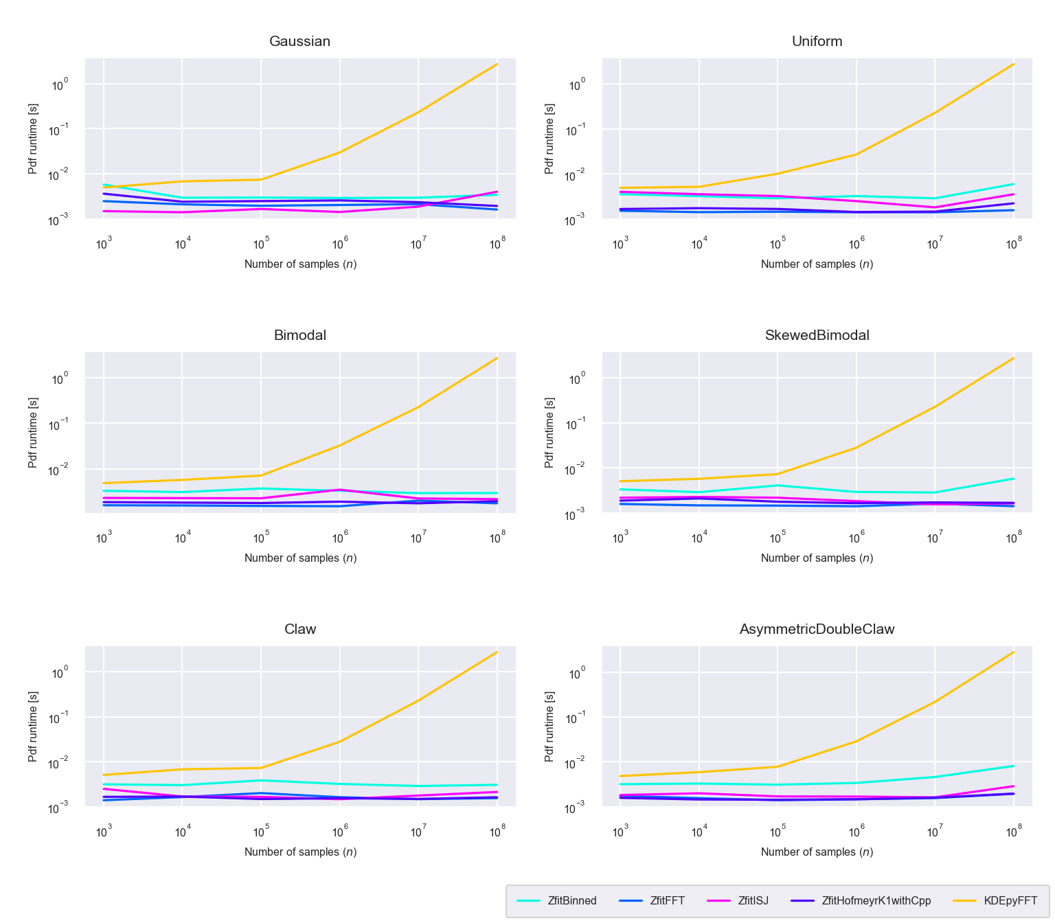
Runtime difference of the evaluation phase between the newly proposed algorithms 'Binned', 'FFT', 'ISJ', 'Hofmeyr' and the FFT based implementation in KDEpy

Figure 5.10: Runtime difference of the evaluation phase between the newly proposed algorithms ‘Binned,’ ‘FFT,’ ‘ISJ,’ ‘Hofmeyr’ and the FFT based implementation in KDEpy

5.4 Comparison to KDEpy on GPU

Now we compare the new methods against KDEpy while leveraging TensorFlow’s capability of GPU based optimization. All computations were executed using two Tesla P100 GPU’s on the openSUSE Leap operating system running on an internal server of the University of Zurich. The number of samples per test distribution is again in the range of $10^3$ - $10^8$. As using the GPU does not change the accuracy, we will only compare the runtimes here. Also the Hofmeyr method is excluded as it was not implemented for running on the GPU.

5.4.1 Runtime

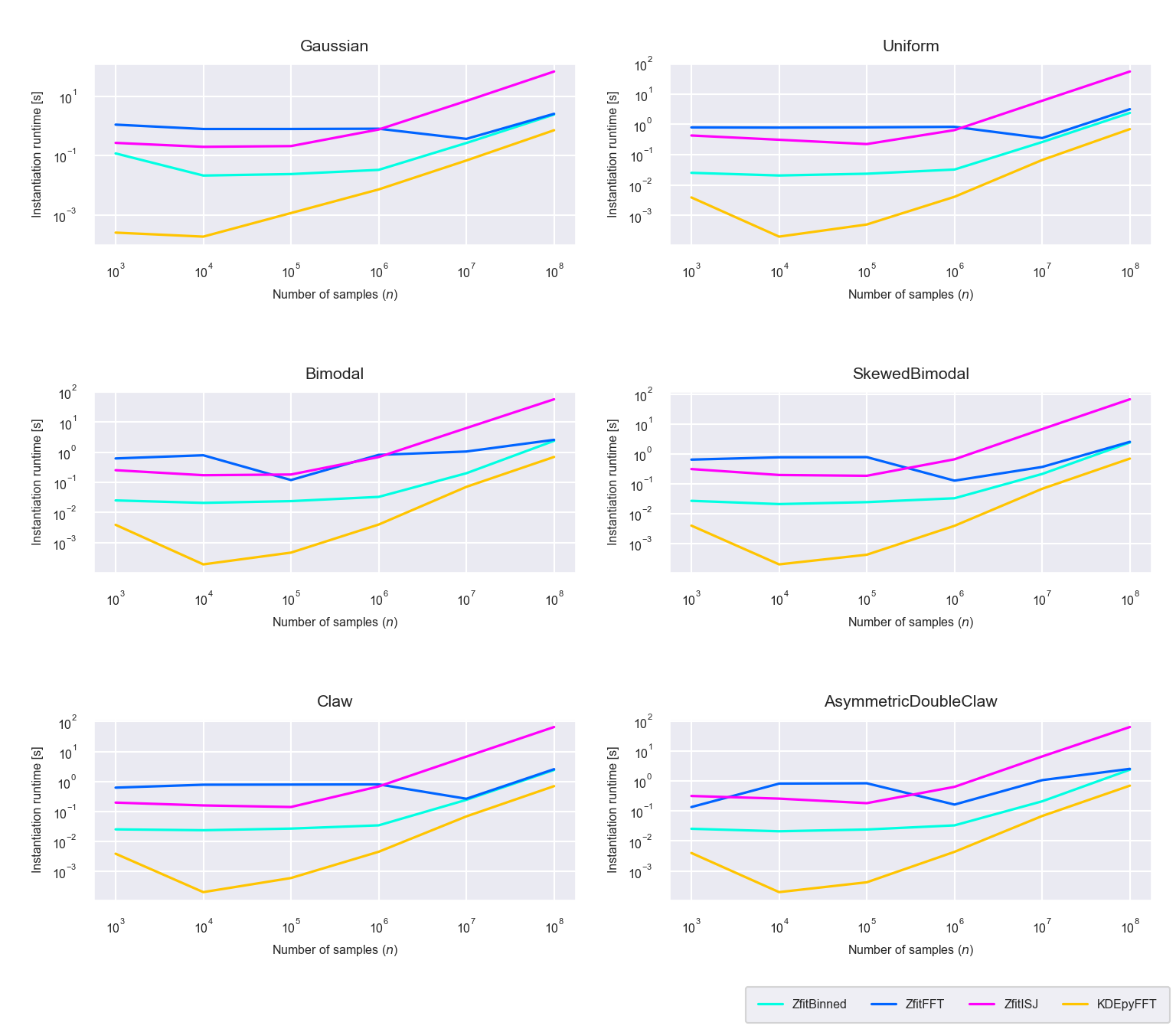
Runtime difference of the instantiaton phase between the newly proposed algorithms 'Binned', 'FFT', 'ISJ' and the FFT based implementation in KDEpy (run on GPU)

Figure 5.11: Runtime difference of the instantiaton phase between the newly proposed algorithms ‘Binned,’ ‘FFT,’ ‘ISJ’ and the FFT based implementation in KDEpy (run on GPU)

The instantiation of the newly proposed implementations runs faster on the GPU than the CPU. This is no surprise as many operations in TensorFlow benefit from the parallel processing on the GPU. For a high number of sample points the newly proposed binned as well as the newly proposed FFT implementation are instantiated nearly as fast as KDEpy’s FFT implementation if run on a GPU (figure 5.11).

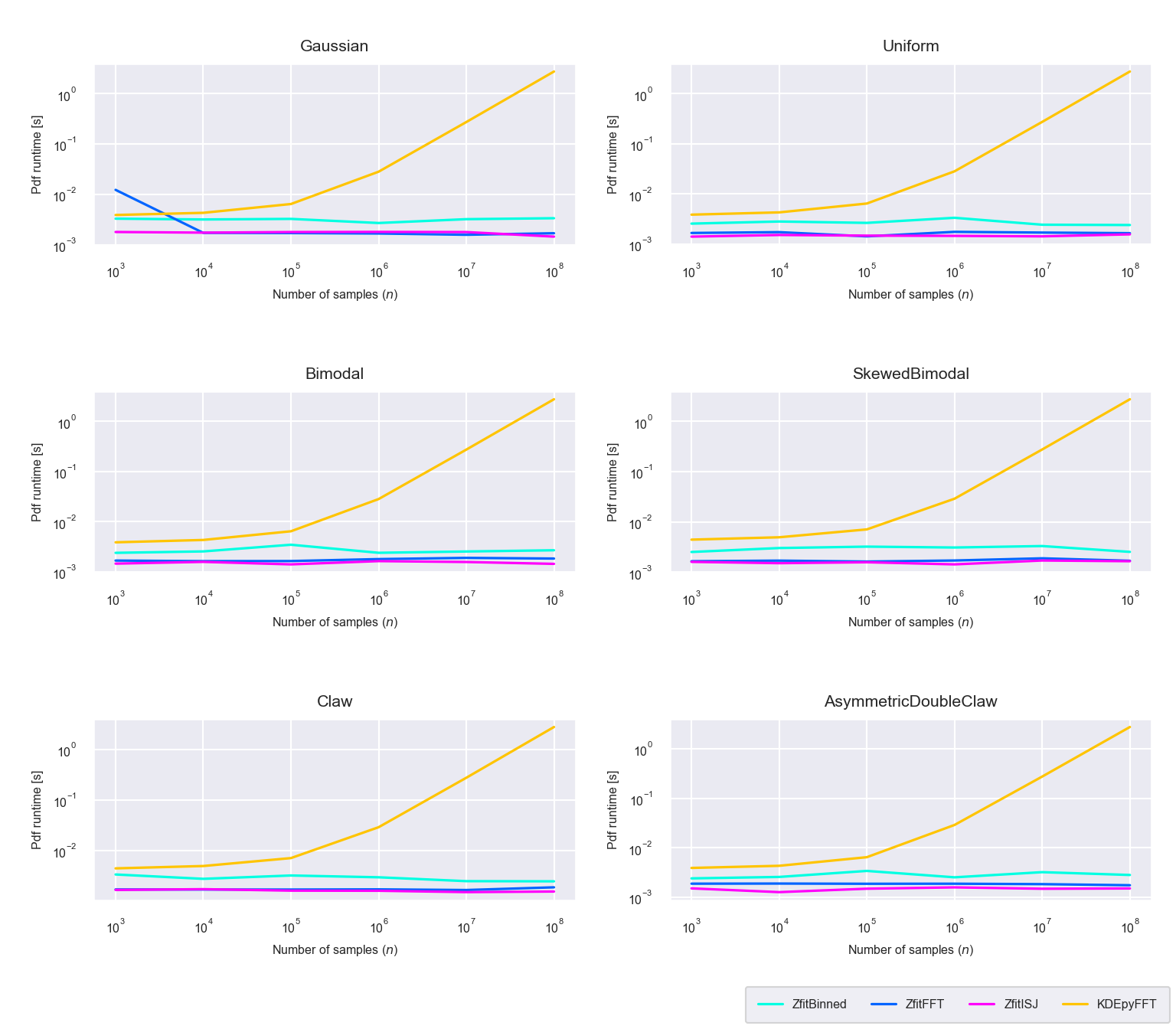
Runtime difference of the evaluation phase between the newly proposed algorithms 'Binned', 'FFT', 'ISJ' and the FFT based implementation in KDEpy (run on GPU)

Figure 5.12: Runtime difference of the evaluation phase between the newly proposed algorithms ‘Binned,’ ‘FFT,’ ‘ISJ’ and the FFT based implementation in KDEpy (run on GPU)

The runtime of the PDF evaluation phase does not differ much from the one seen on the CPU. All new methods are evaluated in near constant time (figure 5.12).

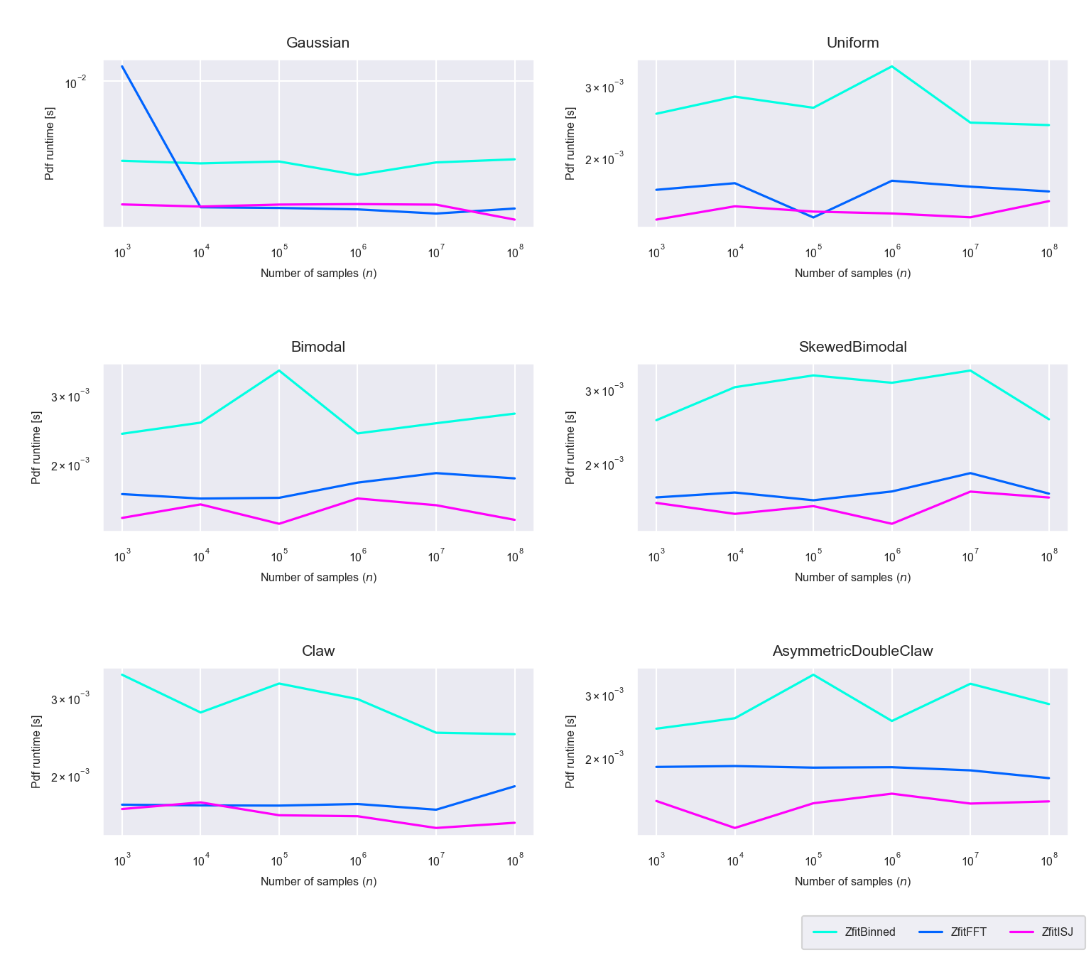
Figure 5.13: Runtime difference of the evaluation phase between the newly proposed algorithms ‘Binned,’ ‘FFT,’ ‘ISJ’ only (run on GPU)

Looking at the evaluation runtimes of only the new methods, we can see that the differences are minimal (figure 5.13) and all evaluation runtimes are of the same order of magnitude.

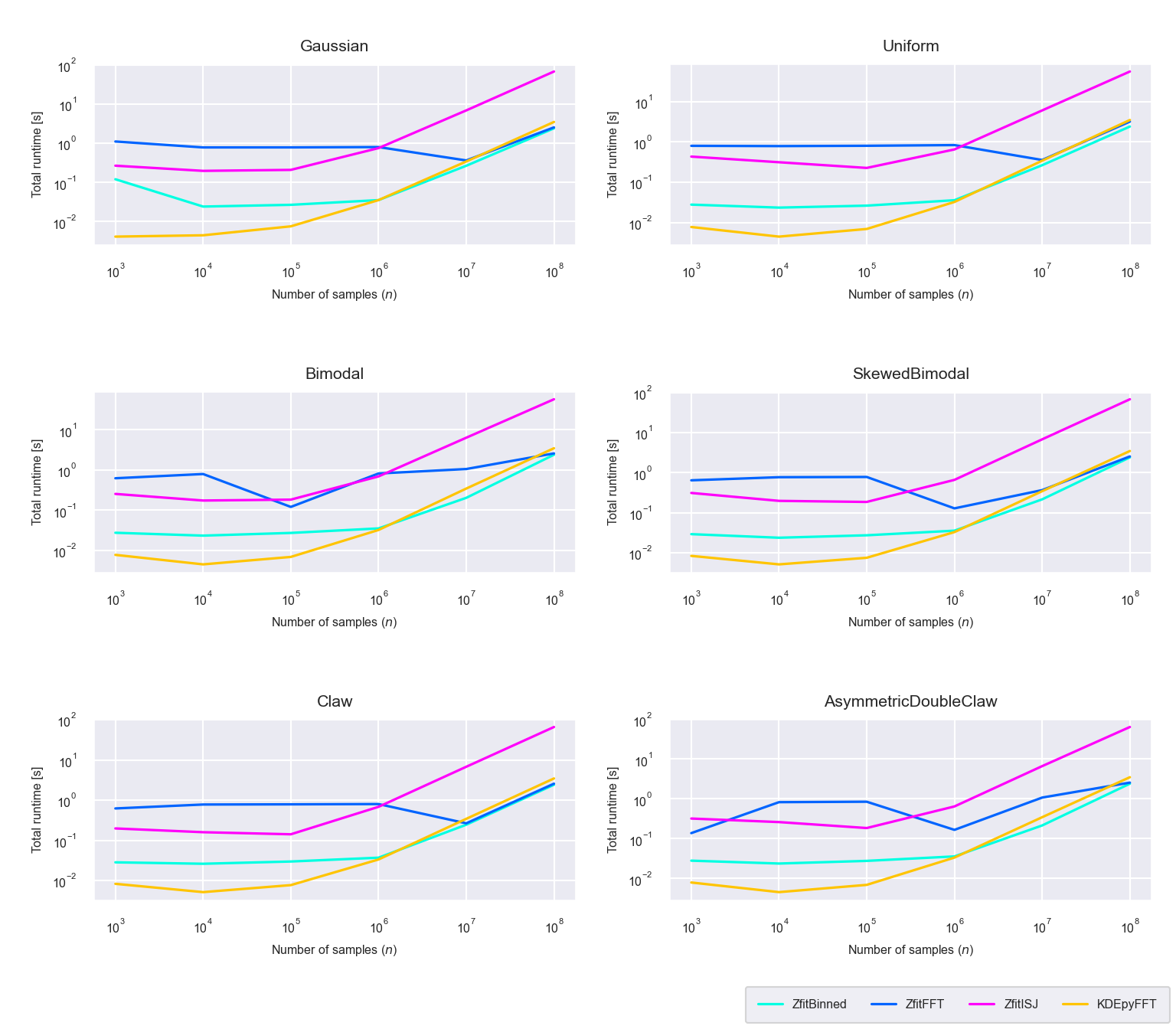
Runtime difference of the total calculation (instantiation and evaluation phase) between the newly proposed algorithms 'Binned', 'FFT', 'ISJ' and the FFT based implementation in KDEpy (run on GPU)

Figure 5.14: Runtime difference of the total calculation (instantiation and evaluation phase) between the newly proposed algorithms ‘Binned,’ ‘FFT,’ ‘ISJ’ and the FFT based implementation in KDEpy (run on GPU)

For larger datasets ($n \geq 10^8$) even the total runtime (instantiation and PDF evaluation combined) of the newly proposed binned and FFT methods is lower than for KDEpy’s FFT method, i.e these new methods based on TensorFlow and zfit can outperform KDEpy if run on the GPU (figure 5.14).

5.5 Findings

The comparisons above lead to four distinct findings.

The Hofmeyr method (ZfitHofmeyr), although a performant algorithm in theory, is difficult to implement efficiently in TensorFlow due to recursion and needs more work to be used for real data.
For use cases where only the evaluation runtime is of importance, for instance in log-likelihood fitting, the newly proposed FFT and ISJ based implementations (ZfitFFT and ZfitISJ) are the most efficient ones.
The ISJ based implementation (ZfitISJ) provides superior accuracy for spiky non-normal distributions by an order of magnitude, while imposing only a minor runtime cost.
For sample sizes $n \geq 10^8$, the newly proposed binned and FFT methods (ZfitBinned, ZfitFFT) are able to outperform KDEpy in terms of total runtime for a given accuracy if run on the GPU.